Thinking about VaR – and not as “Worst Case”

Value at risk or VaR has a bad name. But much of the problem is how we think about and how we talk about VaR. Words do matter and using the wrong terms and phrases often takes us down the wrong road.

The Financial Times, in talking about changes in Morgan Stanley’s VaR model, says that under their VaR model “[Morgan Stanley] expects to lose no more than $63m in a single trading day, within a certain probability”. (“M Stanley shows the ‘flaky’ side of model”, 18 October 2012) This is a common characterization of VaR but the phrase “expect to lose no more” is horribly misleading. A far more instructive way to say the same thing would be “the bank expects to lose more than $63m in a single trading day only infrequently (roughly one day out of 20)”.

This simple change in phrasing is a big improvement and points us in the right direction. First, it emphasizes that Morgan Stanley does expect to lose more than $63m, just not very often. Second, it pushes all of us (regulators, investors, managers) to think about the consequences of losing more than $63m. How much more? How often? How well can Morgan Stanley withstand losses of $63m? The world is an uncertain place and we can never know the maximum loss a firm might suffer. We all need to think carefully about those times when losses are more than the VaR.

This simple change in emphasis – talking about VaR “not as a ‘worst case,’ but rather as a regularly occurring event with which we should be comfortable” (to use Bob Litterman’s words) – goes far towards reminding us all that the proper role of VaR and quantitative risk tools is to inform and educate us about the uncertainty and randomness inherent in our world. There is no certainty in our world, no certainty that a bank will lose no more than $63m. The future is random and contingent and we need to embrace this uncertainty rather than obscure it.

(See my prior post – Rights and Wrongs of VaR – for more detail about how to think about VaR.)

Posted in Risk Management | Leave a comment

Detailed Contents for Quantitative Risk Management

Here is a detailed table-of-contents for my book Quantitative Risk Management – for some obscure reason the book was published without a detailed table-of-contents.

Quantitative Risk Management
A Practical Guide to Financial Risk

Thomas S. Coleman

Detailed Contents as formatted .pdf

CONTENTS
Foreword       ix
Preface       xiii
Acknowledgments       xvii
Part I: Managing Risk       1
Chapter 1: Risk Management versus Risk Measurement       3
   1.1: Contrasting Risk Management and Risk Measurement    5
   1.2: Redefinition and Refocus for Risk Management    5
   1.3: Quantitative Measurement and a Consistent Framework    6
   1.4: Systemic versus Idiosyncratic Risk    12
Chapter 2: Risk, Uncertainty, Probability, and Luck       15
   2.1: What is Risk?    15
   2.2: Risk Measures    19
   2.3: Randomness and the Illusion of Certainty    21
   2.4: Probability and Statistics    39
   2.5: The Curse of Overconfidence    62
   2.6: Luck    64
Chapter 3: Managing Risk       67
   3.1: Manage People    68
   3.2: Manage Infrastructure — Process, Technology, Data    71
   3.3: Understand the Basis    73
   3.4: Organizational Structure    84
   3.5: Brief Overview of Regulatory Issues    90
   3.6: Managing the Unanticipated    92
   3.7: Conclusion    99
Chapter 4: Financial Risk Events       101
   4.1: Systemic versus Idiosyncratic Risk    102
   4.2: Idiosyncratic Financial Events    103
   4.3: Systemic Financial Events    132
   4.4: Conclusion    135
Chapter 5: Practical Risk Techniques       137
   5.1: Value of Simple, Approximate Answers    138
   5.2: Volatility and Value at Risk (VaR)    139
   5.3: Extreme Events    150
   5.4: Calculating Volatility and VaR    153
   5.5: Summary for Volatility and VaR    158
   5.6: Portfolio Tools    158
   5.7: Conclusion    167
Chapter 6: Uses and Limitations of Quantitative Techniques       169
   6.1: Risk Measurement Limitations    170
Part II: Measuring Risk       173
Chapter 7: Introduction to Quantitative Risk Measurement       175
   7.1: Project Implementation    176
   7.2: Typology of Financial Institution Risks    178
   7.3: Conclusion    184
Chapter 8: Risk and Summary Measures: Volatility and VaR       187
   8.1: Risk and Summary Measures    187
   8.2: Comments Regarding Quantitative Risk Measures    202
   8.3: Methods for Estimating the P&L Distribution    206
   8.4: Techniques and Tools for Tail Events    226
   8.5: Estimating Risk Factor Distributions    244
   8.6: Uncertainty and Randomness — The Illusion of Certainty    251
   8.7: Conclusion    254
   Appendix 8.1: Small-Sample Distribution of VaR and Standard Errors    254
   Appendix 8.2: Second Derivatives and the Parametric Approach    262
Chapter 9: Using Volatility and VaR       269
   9.1: Simple Portfolio    269
   9.2: Calculating P&L Distribution    270
   9.3: Summary Measures to Standardize and Aggregate    285
   9.4: Tail Risk or Extreme Events    290
   9.5: Conclusion    306
   Appendix 9.1: Parametric Estimation using Second Derivatives    307
Chapter 10: Portfolio Risk Analytics and Reporting       311
   10.1: Volatility, Triangle Addition, and Risk Addition    312
   10.2: Contribution to Risk    317
   10.3: Best Hedge    327
   10.4: Replicating Portfolio    333
   10.5: Principal Components and Risk Aggregation    337
   10.6: Risk Reporting    346
   10.7: Conclusion    361
   Appendix 10.1: Various Formulae for Marginal Contribution and Volatilities    361
   Appendix 10.2: Stepwise Procedure for Replicating Portfolio    369
   Appendix 10.3: Principal Components Overview    370
Chapter 11: Credit Risk       377
   11.1: Introduction    377
   11.2: Credit Risk versus Market Risk    380
   11.3: Stylized Credit Risk Model    383
   11.4: Taxonomy of Credit Risk Models    409
   11.5: Static Structural Models    411
   11.6: Static Reduced Form Models — CreditRisk+    429
   11.7: Static Models — Threshold and Mixture Frameworks    443
   11.8: Actuarial versus Equivalent Martingale (Risk-Neutral) Pricing    458
   11.9: Dynamic Reduced Form Models    464
   11.10: Conclusion    472
   Appendix 11.1: Probability Distributions    478
Chapter 12: Liquidity and Operational Risk       481
   12.1: Liquidity Risk — Asset versus Funding Liquidity    481
   12.2: Asset Liquidity    484
   12.3: Funding Liquidity Risk    496
   12.4: Operational Risk    513
   12.5: Conclusion    527
Chapter 13: Conclusion       529
About the Companion Web Site       531
References       533
About the Author       539

WILEY
John Wiley & Sons, Inc.

Copyright © 2012 by Thomas S. Coleman. All rights reserved.
Published by John Wiley & Sons, Inc., Hoboken, New Jersey.
Published simultaneously in Canada.

Quantitative Risk Management on Wiley site
Quantitative Risk Management on Amazon

Posted in Publications and Papers | 1 Comment

Risk Management Talk at Greenwich Library

On September 6th 2012 I gave a talk at the Greenwich Library, “How to Think About Risk Management”, co-sponsored by the CFA Society of Stamford. I talked about my views on risk management, focusing on two topics:

  • Arguing for risk management as management – managing people, process, institutions
  • An introduction to the quantitative side – how to think about risk and uncertainty, and what do volatility and VaR (value at risk) really mean?

The talk is based on my book, Quantitative Risk Management. Here are the slides from the presentation, and for those wanting more detail here are the speaker’s notes.

Posted in Conferences, Risk Management | Leave a comment

Graceful Failure and JPMorgan’s Loss

The biggest challenge facing regulators and politicians following the financial crisis is to engineer a regime that allows graceful failure for systemically important financial firms. Failure is, ironically, one of the great strengths of a market-based economy – the creative destruction of Schumpeter. When firms can fail without disastrous social consequences (at least not disastrous for the wider world beyond the owners, investors, workers) then mistakes and bad luck have lower social costs. The real importance of JPMorgan’s recently-announced loss is not the loss – not a seriously damaging event in itself – but the reminder that had it been a serious loss JPMorgan could not have gone out of business without putting the world at risk.

Ironic as it is, a vibrant and functioning economy needs mistakes and failures. Firms need to take risk, need to make mistakes. Risk, mistakes, and bad luck are part of life and without them we would never have the obverse, which is opportunity and success. Most mistakes and most bad luck, in business as in life, are not fatal. Mostly we can compensate, recover from, correct and learn from mistakes. Sometimes, however, mistakes do prove fatal. Some risk and some level of mistakes are necessary in business because without taking the risks we would never have the successes. The key is to find a balance between too much and too little risk. Indeed, the philosopher Nicholos Rescher in his delightful book Luck talks about risk management as “managing the direction of and the extent of exposure to risk, and adjusting our risk-taking behavior in a sensible way over the overcautious-to-heedless spectrum.” (p 187).

In this respect the story in the Financial Times, US and UK eye reaction to bank failure is good news. Regulators are working on “resolution plans” that would see authorities take over a firm and force shareholders and bondholders to take losses, while keeping critical operations open.

I am not optimistic that regulators will be successful, because it is such a difficult problem, but it is the most important piece, maybe the only important piece, of any new regulatory regime. When bank shareholders and bondholders know that their investments are at risk when a firm misbehaves, those investors will monitor and discipline the firm in a way that regulators simply cannot.

Posted in Economics, Musings | Tagged | Leave a comment

Personal Income and Consumption

Summary

I have argued for some time that a robust recovery will occur after households adjust spending downwards. The “savings rate” in the U.S. has risen since the financial crisis, but this reflects changes in taxes, not changes in household behavior.

I believe that households must adjust spending down to reflect levels of lifetime wealth that are lower, after the global financial crises of 2008-2009, than had been expected prior to the crisis. Another way to say the same thing is that households need to adjust their savings upwards to accomplish a long-term deleveraging and readjustment of debt levels

The 2008-2009 recession and the current recovery are all about households de-leveraging and adjusting spending levels downwards relative to income. There are, however, key aspects of the recent past that are often neglected or misunderstood:

  • Starting in 2008 the “Savings rate” rose, particularly after the crisis hit in late 2008.
  • But, the rise in the savings rate from 2008-2010 was almost entirely due to changes in taxes and almost not at all due to changes in household behavior. (See the discussion below on the difference between savings as percent of personal income versus disposable income.)
  • Since early 2010 taxes as a percent of personal income have risen and the “savings rate” has fallen, again almost entirely due to changes in taxes and not household behavior.

Note that any rise in the “savings rate” due to lower taxes is not really an adjustment in household behavior or overall debt profile. Increased government debt will eventually have to be repaid through future higher taxes.

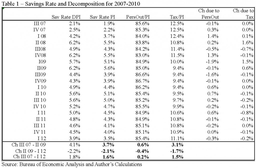
Table 1 shows the current savings rate and spending rates (quarterly) during and subsequent to the recession. A few points to note:

  • From 2007:QIII through 2009:QII
    • The savings rate (as percent of personal income – see discussion below) rose by 3.7 percentage points
    • If this 3.7 percentage point rise, 3.1 percentage points was due to lower taxes
  • From 2009:QII through 2012:QI
    • The savings rate has fallen by 2.1 percentage points
    • Of which 1.7 percentage points was due to higher taxes (and 0.4 points due to higher household outlays)
Table 1

Table 1 – Savings Rate and Decomposition for 2007-2010

If, as I think may happen, taxes rise modestly and also households do eventually adjust spending down, there will be a recession. This could, however, set the stage for a robust recovery to follow.

Since the bubble burst in 2007-2008 all forms of wealth have fallen – falling housing prices have reduced real estate holdings; stock markets have fallen or stagnated; and, probably most importantly, employment and prospects for future earnings have fallen. The fall in lifetime wealth should naturally induce some adjustment in household spending. The recession was simply that adjustment of spending to new levels of perceived wealth.

I don’t think the imbalances that led to the financial crisis of 2007-2009 are fully redressed (at least in the US). Spending is supported by low taxes (an explicit government policy to ameliorate the recession of 2008-2009). Eventually taxes will have to rise to fund the government deficit, and this will put pressure on spending. Either the savings rate will fall (building future imbalances) or spending will fall (recession).

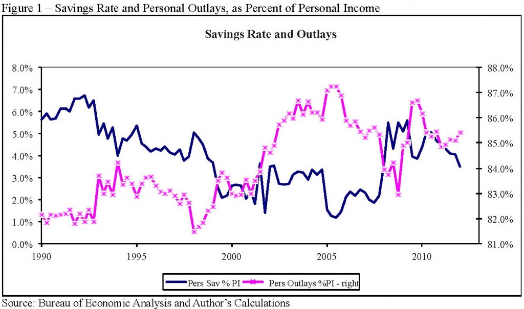
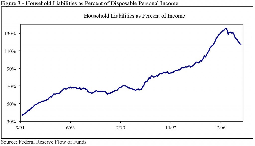
Longer-term trends (over the past two decades) are shown in figures 1, 2, and 3:

  • Savings rate (more accurately, what is left over from current spending) fell from roughly 6% of income to below 2% in 2007/2008 and rebounded to almost 6% by early 2009.
  • Taxes rose during the late 1990s but fell dramatically post-2000, and again in 2008/2009.
  • Spending has risen from about 83% of income (1990s) to over 87% in 2005 and is now roughly 86%. It is still high by historical standards and supported by low taxes, even if not as high as during the bubble.
    • Household liabilities (measured in the Federal Reserve’s quarterly flow of funds reports) have fallen since 2007, from 135.1% of income in 2007:QIII to 117.5% in 2011:QIV. This is good news and shows households have started de-leveraging. Unfortunately the increase in government debt has been far larger. According to the OECD, central government debt for the US grew by $3.98tn from 2007 to 2010, or from 35.7% of GDP to 61.3%. Future tax liabilities, which are a future liability and thus function as a sort of implicit household debt, have probably offset any decrease in directly-owned household debt. The net result is that household leverage has probably not decreased much, if at all, over the past three years.

      Figure 1

      Figure 1 – Savings Rate and Personal Outlays, as Percent of Personal Income

      Figure 2

      Figure 2 – Current Personal Taxes, as Percent of Personal Income

      Figure 3

      Figure 3 - Household Liabilities as Percent of Disposable Personal Income

      Decomposition of Movements in Spending and the Savings Rate

      Table 1 shows the savings rate. The definitions of savings and spending rates, together with a decomposition of savings as a percent of personal income, are discussed here.

      Economists commonly consider the “savings rate,” which is the difference between current income and spending – the excess of income left after spending and taxes are accounted for. The definition is:

      Savings Rate = (Disposable Personal Income – Personal Outlays) / Disp Pers Inc .

      (This “savings rate” is not exactly savings as one usually thinks of savings, but rather a definition of the excess of income over spending in the aggregate economy. One could equally well talk of the “spending rate” – Outlays / Income – which is just one minus the “savings rate”.)

      It is useful to decompose the rise in the savings rate in order to understand it a little more. To do so it is useful to consider savings as a percent of total personal income. Basically,

      Disposable Personal Income = Personal Income – Personal Current Taxes
      Savings = Disposable Personal Income – Personal Outlays

      The standard definition of the savings rate is savings divided by Disposable Income:

      Savings Rate (DPI) = (Disposable Personal Income – Personal Outlays) / Disp Pers Inc
      = 1 – Personal Outlays / Disp Pers Inc

      We can, however, define a savings rate divided by personal income that is only slightly different:

      Savings Rate (PI) = (Personal Income – Personal Current Taxes – Personal Outlays) / Pers Inc
      = 1 – Pers Curr Taxes / Pers Inc – Pers Out / Pers Inc

      Since DPI and PI differ only by Pers Curr Taxes, which has monthly changes that are not large relative to the level of DPI and PI, the two measures will be very much the same. The advantage of the second is that we can decompose changes in that savings rate into changes due to taxes and that due to changes due to outlays (spending).

Posted in Economics, Musings | Leave a comment

Risk, Black Swans, and Brown Turkeys

The mathematics of volatility and VaR alone are just not enough for understanding risk in today’s environment. We are living in extraordinary times – probably the most extraordinary in three generations. (Don’t get me wrong – I’m not arguing that we should throw out the mathematics and the quantitative tools. Unlike many others – there is a minor industry blaming all our current travails on the evils of VaR – throwing out the mathematics is patently absurd.)

But the risks today are really macroeconomic, political, policy risks, systemic risks; not the risks that an individual firm will run into trouble (JPMorgan’s recent loss notwithstanding). The risks are the big, existential risks of sovereign debt default, currency devaluation and debasement, inflation.

But we need to put all this in an historical perspective. We’ve been here before, in fact many times. It seems new and strange only because our collective memory is short. Our current situation may seem extraordinary by comparison with the past 10 or 20 years, but when we look further back in history, when we take a 100 or 200 year perspective, today’s events are not extraordinary after all.

My presentation at the conference on U.S. Expatriate Investing: Risk vs. Reward in an Uncertain World in January 2012 tried to put some of our current travails in an historical perspective. Why the title Risk, Black Swans, and Brown Turkeys? People talk about “Black Swans” – unpredictable and inherently unforeseen events – events that because of their unpredictability have a major impact. The term traces back to Juvenal, in Latin “rara avis in terris nigroque simillima cygno”. In English “a rare bird in the lands, and very like a black swan”. Originally meaning something that was patently impossible (since all known swans were white) it has come to mean supposedly impossible events which, when observed, completely up-end received wisdom.

But the term “Black Swan” is horribly over-used. There may be Black Swans out there, but let me assure you that the financial crisis that started in 2007 and continues today with the eurozone crisis is not a Black Swan. Before-hand it was impossible to predict when or even if the bubble would burst. But crises such as we are living through have been common throughout history and the current one has been absolutely no surprise to those who study such events. The current crisis would seem very familiar to a London banker living through the Barings crisis of 1890 (yes, Barings went under in 1890 as well as 1995) or a New York stock-broker during the crisis and panic of 1907-08.

Today’s events are better characterized as “Brown Turkeys” – events that are unpredictable, surprising when they occur, but are out there if you know where to look. If you have ever tried to hunt turkey you will know that they rarely show their face, particularly when you are hunting them. But the woods are full of them. (At least at my father’s place in West Virginia.) They are there, we just don’t see them. But just because they aren’t in our front yard every day doesn’t mean they don’t exist. We can’t predict when we’ll find one and it may be a huge surprise when we finally get one within shot, but only a fool would be surprised that they actually exist. We can’t predict when or where we might come across a Brown Turkey but any knowledgeable hunter knows they’re out there.

Read more in the slides (.pdf) or read through the complete lecture notes (20 pages, .pdf).

Posted in Economics, Musings | Leave a comment

JPMorgan Chase loss seems to be an idiosyncratic trading loss

The JPMorgan Chase loss seems to be a plain-vanilla trading loss – unfortunate and bad news, but not a sign of something more serious in the financial system. Bad as they are, we have lived with these kind of trading losses for decades.

Details about the loss announced by JPMorgan last week are sketchy, but what I can discern tells me that it is more akin to a standard trading loss (an idiosyncratic loss, having to do with specific issues at JPMorgan) than a systemic loss (related to macroeconomic or financial system issues).

There is a long history of trading losses at financial firms, and studying these losses both helps us to understand the sources and responses to such events, and also helps put this specific event into perspective.

The announced $2bn loss is large, but by no means the largest – LTCM in 1998 was $4.60bn, Amaranth Advisors $6.50bn in 2006, and Société Générale $7.22bn in 2008 – and were we to adjust for inflation and growth in the economy those would be even larger today. And LTCM and Amaranth were small compared with today’s Morgan Chase. According to the Financial Times the portfolio within Morgan Chase that suffered the loss was $360bn, so although $2bn is large in absolute terms it is only 0.6% of the portfolio – this does not minimize the loss but again helps put it in perspective.

When we examine trading losses over the years, two facts become apparent:

  • They occur more regularly than we would like to think
  • The sources and reasons are varied, but most are not “rogue traders”, and transparency and mark-to-market matter

In chapter 4 of my recent book (Quantitative Risk Management published by Wiley, also available in the CFA monograph
A Practical Guide to Risk Management, available for free download)
I examine 35 cases of trading losses over the years, ranging from the large and well-known (LTCM’s collapse in 1998) to the smaller and more obscure (traders at National Australia bank losing $310mn in 2004 on FX trading). Fully 40% involved no fraud, and only 26% involved fraudulent trading that fits our image of the rogue trader. Many cases originated in standard business which either went badly wrong (for example Metallgesellschaft in 1994 where a poorly-designed hedge against oil prices went disastrously wrong, or Askin Capital Management, also in 1994, where investments in principal-only securitized mortgage securities lost heavily when interest rates rose) or got out of control (Aracruz Celulose and Sadia, where FX hedging apparently morphed into outsize speculation).

One lesson we can take from examining these cases is something which should be blindingly obvious – financial markets are risky and sometimes bad luck happens. Investors and managers often make mistakes and foolish decisions, but sometimes there is simple bad luck. Personally, I think LTCM made foolishly large one-way bets on swap spreads and long-term equity volatility, but they undoubtedly suffered the bad luck of having Russia default on its debt at a time when the financial markets were somewhat unsettled. (In fact, a friend of mine escaped the Russian debacle only because she had the good luck to forget to roll an expiring position in Russian bills when they came due on a Friday and thus owned no bills at the time of default.)

Financial markets are risky and bad things do happen, and so transparency and mark-to-market are vitally important. When losses do not come to light quickly they tend to grow. It is human nature to avoid bad news. Case after case shows the danger of allowing losses to sit and the all-too-human tendency to try and fix the problem, try to trade out of the loss. JPMorgan has at least owned up to the loss with some alacrity.

One final lesson we should take from examining idiosyncratic trading losses is that they are bad, but pint-sized relative to losses from systemic events. Consider Hypo Group Alpe Adria (discussed on p. 120 in the CFA monograph, p. 132 in the Wiley book). They had an idiosyncratic loss of eur 300mn in 2004 related to a currency swap. But then they got caught in the global financial crisis, and in December 2009 had to be rescued by the Republic of Austria – after-tax loss of eur 1,600mn for 2009. Another example – Dexia Bank – idiosyncratic loss of eur 300mn in 2001, but losses for 2008 of eur 3,300mn (and more recent nationalization). And don’t forget Fannie Mac and Freddie Mac – as of May 2010 the US government had provided $145bn of support, and it has only grown since then. Idiosyncratic losses are measured in the hundreds or million dollars, maybe a couple billion. Systemic losses start in the billions and run to the hundreds of billions. Idiosyncratic are one or two orders of magnitude smaller than systemic. Idiosyncratic losses can bring down a single firm. Systemic events can bring down a nation.

We should remember that the loss JPMorgan announced last week is firmly in the category of idiosyncratic loss, rather than systemic. The discussion of reasons and responses should be related to the nature of that idiosyncratic loss. Unfortunately, much of the discussion has been, and will continue to be, around regulation and responses for systemic risk.

Posted in Musings, Risk Management | Tagged | Leave a comment

Rights and Wrongs of Value at Risk (VaR)

With the loss announced by JPMorgan Chase last week there are, once again, loud and varied denunciations of Value at Risk or VaR. Unfortunately, such talk sheds little light upon and often shows misunderstanding of the underlying issues.

Take the statement from the Lex Column of the Financial Times from Monday, May 14th:

Why does VaR seem limited almost to the point of uselessness? One reason is that it does not offer an absolute guarantee that it will do what it says on the tin. It represents the potential losses in a trading portfolio over a given period of time at a given level of confidence. That covers almost all eventualities. The trouble is that problems usually arise in the ones that are not covered.

First, let’s start with that “absolute guarantee”. Anybody remotely acquainted with financial markets, and the writers of the Lex Column in particular, should know that there are no “absolute guarantees” in financial markets, or in life for that matter. (Except, maybe, for death and taxes. Although some politicians seem to be working on taxes.)

VaR only promises to give an estimate of the minimum or typical amount we might lose on the worst trading day during, say, a year. It doesn’t represent the worst loss we might suffer. In financial markets, whatever our worst-case scenario, something worse will happen sometime, somewhere. Although some authors talk about VaR as the “statistically worst-case loss,” this is a horribly misleading idea. VaR should be viewed as a periodically occurring event that, while not likely, we should be perfectly comfortable with. We should think of VaR as providing a scale for possible large losses, not a maximum loss or worst-case scenario.

Let’s examine what VaR says it will do “on the tin”. Doing so takes a little bit of work but we will be well-rewarded by better understanding of what VaR can or cannot do.

Financial risk is in some ways so simple, because it is all about money – profit and loss and the variability of P&L. What do we mean by P&L and the variability of P&L? Start with a very simple financial business, betting on the outcome of a coin flip. We make $10 on heads and lose $10 on tails. We could graph the P&L distribution as in panel A of Figure 1. The probability is one-half of losing $10 and one-half of making $10.
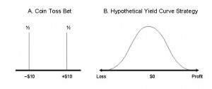
Sample Distributions

Figure 1 - Examples of Simple P&L Distributions

This kind of distribution shows us the possible outcomes (possible losses and gains along the horizontal) and how likely each of these is (probability along the vertical). This is fundamental to how we think about financial risk – it shows us the possible profits or losses.

In fact, this distribution is what we mean by financial risk – the possibility that we may make money but also may lose money.

There are two issues we need to discuss regarding this distribution. First, we would like some simple way to summarize this distribution. That is where VaR comes in. VaR is simply a point on the left hand side of the distribution. Look at Figure 2 – the VaR is the point on the distribution labeled “$215,000”. We have simply chosen a point on the left hand part of the distribution, where there is 5% chance that the loss will be worse.
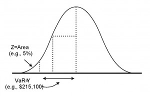
VaR and P&L distribution

Figure 2 - P&L Distribution for a US Treasury Bond, Showing the VaR

In other words, there is a 5% or 1/20 chance that the loss will be worse than $215,000. This is why I say the VaR is the “minimum or typical amount we might lose” – in this case on the worst trading day out of 20. If we chose 0.4% instead of 5% the point would be further out on the left, and then the VaR would be the minimum or typical amount we might lose on the worst trading day in a year (worst out of 250 days).

But look at the figure – it is easy to see things could be worse, that there are losses further out to the left. The VaR never tells us the worst that could happen – it only sets the typical bad day (out of 20 days for 5%, out of 250 days for 0.4%). Things can always get worse, so if we see something worse than the VaR that may be the result of simple bad luck.

There is a more fundamental issue with the distribution, however. We never know the distribution with certainty. We never can know the future, but the distribution we care about is the distribution of profit and loss over the coming days, weeks, or months. We can never know this distribution with any certainty. We can estimate, make a guess at it, but we never can know it for certain.

But we have to learn to live with uncertainty, randomness, luck. The world is full of uncertainty, assumptions, guesses, and estimates. That is life. Yes, we have to make sure our estimates and assumptions are good and reasonable, but we can find no “absolute guarantees” in this world. When the Financial Times says “It [VaR] is based on assumptions, uses historical data …” that cannot be a criticism – it is simply stating the obvious. Anyone who does not like the uncertainty, the assumptions, should probably not be in business.

There is one final and fundamental problem with VaR, an existential problem to which there is no solution. That problem is extreme or tail events, outliers.

The loss at JPMorgan is an outlier, an extreme event. VaR, and quantitative risk measures in general, do not catch extreme events. But extreme events are, by their very nature, difficult to quantify. Experience does not catch extreme events. Imagination can try, but even that fails. Extreme events are extreme and hard to predict, and that is just the way life is. We need to recognize this limitation, but it is hardly a failure of VaR or quantitative techniques. To criticize VaR and the field of risk measurement because we cannot represent extreme events is just silly, like criticizing the sky because it is blue. Anybody who does not like extreme events should not be in the financial markets. Luck, both good and bad, is part of the world. We can use quantitative tools to try to put some estimates around extreme events, but we have to learn to live with uncertainty, particularly when it comes to extreme events.

There is much more, about VaR, volatility, extreme events, and other quantitative risk issues in my new book, Quantitative Risk Management published by Wiley.

Posted in Musings, Risk Management | Tagged , | Leave a comment

JPMorgan Chase loss and idiosyncratic vs. systemic risk

The loss announced by JPMorgan Chase last week raises many interesting questions, one being the distinction between idiosyncratic and systemic risk. The distinction between idiosyncratic risk versus systemic risk (and idiosyncratic vs. system events) is vitally important because the sources of and the responses to the two are quite different. Unfortunately the distinction is often ignored, particularly in popular and political discussions. Sometimes it seems people intentionally confuse them.

Quoting from chapter 1 of my recent book:

Idiosyncratic risk is the risk that is specific to a particular firm, and systemic risk is widespread across the financial system. The distinction between the two is sometimes hazy but very important. Barings Bank’s 1995 failure was specific to Barings (although its 1890 failure was related to a more general crisis involving Argentine bonds). In contrast, the failure of Lehman Brothers and AIG in 2008 was related to a systemic crisis in the housing market and wider credit markets.

The distinction between idiosyncratic and systemic risk is important for two reasons. First, the sources of idiosyncratic and systemic risk are different. Idiosyncratic risk arises from within a firm and is generally under the control of the firm and its managers. Systemic risk is shared across firms and is often the result of misplaced government intervention, inappropriate economic policies, or exogenous events, such as natural disasters. As a consequence, the response to the two sources of risk will be quite different. Managers within a firm can usually control and manage idiosyncratic risk, but they often cannot control systemic risk. More importantly, firms generally take the macroeconomic environment as given and adapt to it rather than work to alter the systemic risk environment.

The second reason the distinction is important is that the consequences are quite different. A firm-specific risk disaster is serious for the firm and individuals involved, but the repercussions are generally limited to the firm’s owners, debtors, and customers. A systemic risk management disaster, however, often has serious implications for the macroeconomy and larger society. Consider the Great Depression of the 1930s, the developing countries’ debt crisis of the late 1970s and 1980s, the U.S. savings and loan crisis of the 1980s, the Japanese crisis post-1990, the Russian default of 1998, the various Asian crises of the late 1990s, and the worldwide crisis of 2008, to mention only a few. These events all involved systemic risk and risk management failures, and all had huge costs in the form of direct (bailout) and indirect (lost output) costs.

It is important to remember the distinction between idiosyncratic and systemic risk because in the aftermath of a systemic crisis, the two often become conflated in discussions of the crisis. Better idiosyncratic (individual firm) risk management cannot substitute for adequate systemic (macroeconomic and policy) risk management. Failures of risk management are often held up as the primary driver of systemic failure. Although it is correct that better idiosyncratic risk management can mitigate the impact of systemic risk, it cannot substitute for appropriate macroeconomic policy. Politicians—indeed, all of us participating in the political process—must take responsibility for setting the policies that determine the incentives, rewards, and costs that shape systemic risk.

This is from chapter 1 of
Quantitative Risk Management published by Wiley (also available in the CFA monograph
A Practical Guide to Risk Management, available for free download as .pdf, EPUB, iBookstore, or as Kindle from Amazon

Posted in Musings, Risk Management | Leave a comment

Quantitative Risk Management

Published by Wiley in May 2012, this book presents a road map for tactical and strategic decision-making designed to control risk and capitalize on opportunities, covering the techniques and tools used to measure and monitor risk. These techniques and tools are often mathematical and specialized, but the ideas are simple. The book starts with how we think about risk and uncertainty, then turns to a practical explanation of how risk is measured in today’s complex financial markets.

  • Covers everything from risk measures, probability, and regulatory issues to portfolio risk analytics and reporting
  • Includes interactive graphs and computer code for portfolio risk and analytics
  • Explains why tactical and strategic decisions must be made at every level of the firm and portfolio

This volume, in common with the CFA monograph A Practical Guide to Risk Management, focuses on how to think about risk, but also includes the technical material necessary to actually measure risk.

Providing the models, tools, and techniques firms need to build the best risk management practices, Quantitative Risk Management is an essential volume from an experienced manager and quantitative analyst.

Here is a detailed table-of-contents.

Here are links for purchase (at Amazon, Barnes and Noble, etc.), and here is a link to the Wiley.com site, with more description and excerpts.

Posted in Publications and Papers, Risk Management | Tagged | Leave a comment