
Last week I was talking to a group of risk professionals and advocating marginal contribution to risk when someone asked “what about calculating marginal contribution to VaR for historical or Monte Carlo simulation?” (NB – we’re talking here about Litterman’s marginal contribution, the contribution for a small or marginal change in an asset holding – RiskMetrics calls it “incremental VaR” and they use the term “marginal VaR” for completely removing an asset from the portfolio – but that’s not a “marginal” change. Oh well. See Exhibit 5.2 of the free download A Practical Guide to Risk Management or p 317 ff of my Quantitative Risk Management.)
I happen to think marginal contribution is one of the most useful portfolio tools for managing risk. One can calculate marginal contribution to volatility, or VaR, or expected shortfall – in fact contribution for any linearly homogeneous risk measure. It is easy to write down the formula for contribution to volatility and VaR (see my book Appendix 10.1, pp 365-368 or McNeil, Frey, Embrecht’s Quantitative Risk Management equations 6.23-6.26). When estimating by parametric (also called delta-normal or variance-covariance) calculating contribution to volatility or VaR is fast and easy.
But for simulation (historical or Monte Carlo) contribution to VaR has some severe problems. Contribution to volatility is still straight-forward, and the sampling variability of the estimate will go down as we increase the number of trials in the simulation. Not for contribution to VaR – the sampling variability of the estimate is large and will not go down as we increase the number of repeats or draws for the simulation. A longer simulation does not give a more precise estimate of the contribution to VaR.
The problem is that the contribution to VaR for an asset depends on the single P&L draw that happens to be the alpha-th P&L observation for the portfolio (the simulated alpha-VaR). The contribution to VaR depends on that single P&L observation in such a way that the sampling variability does not change with the number of trials in the simulation. (I run through a simple example on p 367 that may make this a little more clear. (But the sentence in the middle of the page should read “For Monte Carlo (with correlation rho=0) there will be a 10 percent probability that the marginal contribution estimate is outside the range [0,1], when in fact we know the true contribution is 0.5.”))
BUT there may be a work-around – what we might call the “implied contribution to VaR”.
- According to McNeil, Frey, Embrecht’s Quantitative Risk Management (p260) the marginal contribution to VaR will be proportional to the marginal contribution to volatility for any elliptical distribution. (Same for expected shortfall.) And the class of elliptical distributions is pretty large – beyond the normal it includes fat-tailed and even distributions having no higher moments: Student-t, simple mixture of normals, Laplace, Cauchy, exponential power.
- This may provide a way to get marginal contribution for VaR under simulation, as follows:
- Calculate marginal contribution to volatility – this will be relatively well estimated by simulation since it depends on the variances and covariances. The sampling variation can be made small by increasing the number of repeats in the simulation. Call this the marginal contribution to vol in levels – MCvolL
- Divide through by the value of the volatility – call this new variable the marginal contribution to volatility in percent – MCvolP
- According to McNeil, Frey, Embrecht the MC to vol and to VaR will be proportional (as long as P&L distribution is elliptical), so that MCvolP = MCvarP
- You can now get the marginal contribution to VaR – multiply MCvarP by the estimated VaR: MCvarL = VaR * MCvarP = VaR * MCvolP
- The alternative (which I suggest in the appendix but which has some obvious problems) is to run multiple complete simulations:
- For each simulation calculate marginal contribution to VaR
- Average across simulations
- There are two big problems with this. First it is very expensive – having to run a large number (hundreds or thousands) of complete simulations. Second, for historical simulations you only have one set of draws – the history. (Unless you bootstrap using the historical observations or in some other way use the historical data to create the distribution from which you draw for Monte Carlo – but this might be a good idea anyway.)
- Note, however, that each simulation can be pretty short, since the sampling variability of the estimated contribution to risk does not really change with the number of repeats
- Another alternative is to use a few of the P&L simulations just around the alpha-VaR simulation, and then average the contribution-to-VaR estimates. You can arrange so that the sampling variability will go down as the number of draws increase. But the sampling variability will still be large.
Let’s look at some simulation results. Take two assets, X1 and X2, each normally distributed with mean zero, portfolio weight 1/2, uncorrelated, and variance 2 (so that the portfolio variance will be 1). The volatility will be 1.0 and the 5% VaR will be 1.645. The marginal contribution (proportional) will be 1/2 for each asset and both contribution to volatility and VaR. The contribution to volatility in levels is 1/2 for each asset, the contribution to VaR 0.82 for each.
In a simulation we would pick the length – the number of normally-distributed (X1, X2) pairs to draw. I will consider two cases – length 500 and 2000. “Length 500” means we draw 500 (X1, X2) pairs and for each of these 500 pairs calculate the P&L as the sum of X1 and X2. With these 500 simulated P&Ls we can then calculate the volatility (the standard deviation from the 500 observations), the 5% VaR (the 25th-smallest observation), and the marginal contribution to volatility and VaR using the appropriate formulae. But here we are particularly interested in how these measures (volatility, VaR, marginal contribution to volatility and VaR) randomly vary from one simulation to another. Thus I will run the complete 500-pair simulation multiple times – 10,000 times – and calculate the sample standard deviation of the measures (over the 10,000 repeated simulations).
I am also interested in what happens when the original simulation length increases from 500 pairs to 2000 pairs – when we increase the original simulation length by a factor of 4. We should expect our simulated measures to be less variable – the sample standard deviation of volatility, VaR, etc. should go down by a factor of 2 – the usual root-n behavior of Monte Carlo.
The following shows the results for simulations of length 500 and 2000, and repeating the complete simulations 10,000 times.
| Length 500 | Volatility | MC Vol Level | MC Vol Prop’l | 5% VaR | MC VaR Level | MC VaR Prop’l |
| Mean | 1.00 | 0.50 | 0.50 | -1.65 | -0.83 | 0.50 |
| Std Dev | 0.032 | 0.028 | 0.023 | 0.095 | 0.507 | 0.307 |
| Length 2000 | Volatility | MC Vol Level | MC Vol Prop’l | 5% VaR | MC VaR Level | MC VaR Prop’l |
| Mean | 1.00 | 0.50 | 0.50 | -1.65 | -0.83 | 0.50 |
| Std Dev | 0.016 | 0.014 | 0.011 | 0.047 | 0.504 | 0.306 |
Notice that the sampling variability for the volatility, 5% VaR, and contribution to volatility (the standard deviation over the 10,000 repeated simulations) goes down by 2 as we go from a simulation of 500 to 2000. This is exactly what we expect – the number of repeats goes up by 4 and the sampling variability goes down by 2 – this is the root-n of Monte Carlo. But the sampling variability does not go down for the contribution to VaR – it does not change with the length of the simulation.
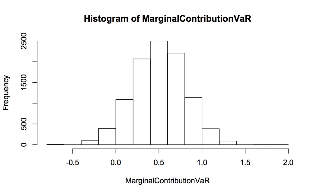
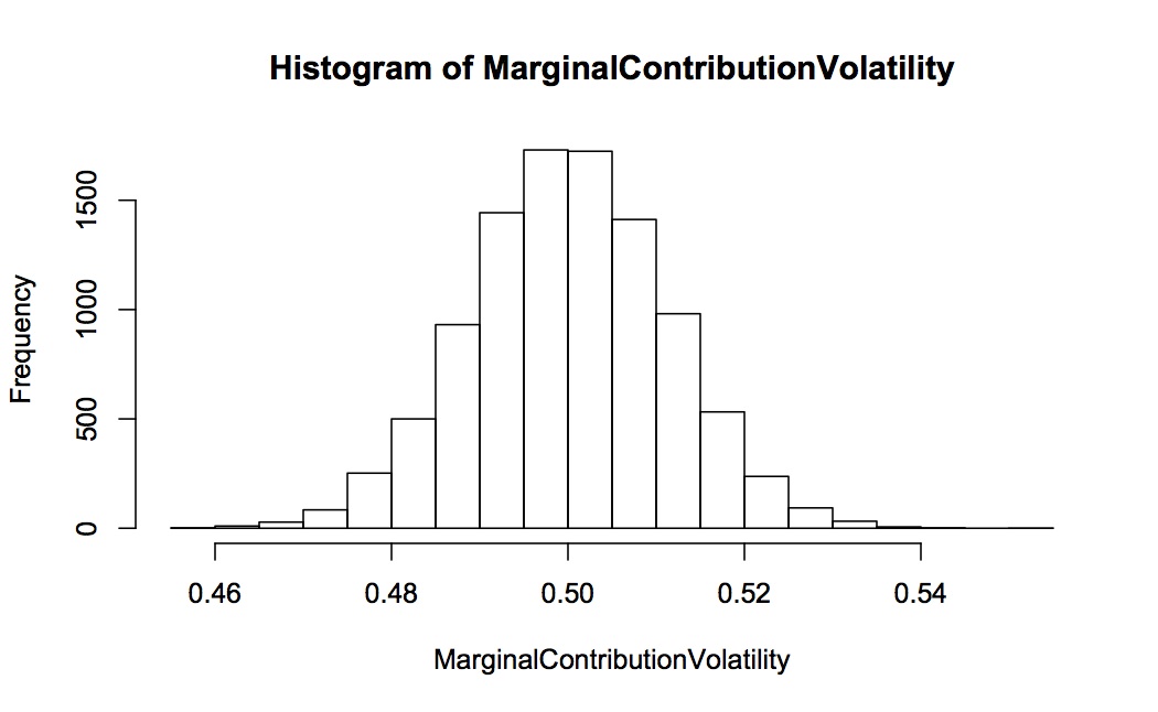
The following two graphs show the histogram for the estimated marginal contribution to volatility and VaR for asset 1 (both proportional, so each is expected to be 0.5). This is for 10,000 complete simulations, each simulation 2000 long. Notice how spread out the distribution of contribution to VaR is relative to contribution to volatility – they are on completely different scales with contribution to VaR going from -0.5 to +2.0 and contribution to volatility only 0.46 to 0.54.
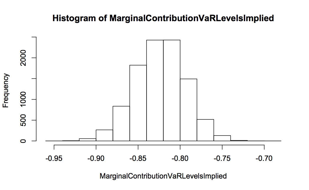
We can also look at the contribution to VaR in levels. Again, this is for 10,000 repeated simulations, each simulation 2000 long. The distribution of the simulated contribution to VaR is shown in the first histogram – the expected value is -0.82 but the spread is huge with considerable mass as down to -2 and up to +0.5. In contrast the implied contribution to VaR (calculated from the proportional contribution to volatility as outlined above) is very well-behaved with virtually all the mass between -0.9 and -0.75.

This simulation shows pretty dramatically the problems with estimating contribution to VaR by simulation, and how the idea of “implied contribution to VaR” solves this problem. OK, you might argue that this simulation is only for two assets and is based on normality. But the proportionality between contribution to volatility and VaR holds for a wide class of distributions (elliptical, which includes Student-t, mixture of normals, Cauchy, Laplace, exponential power) so this technique is likely to work more widely.
In the end, however, I generally look at volatility more than VaR. (One big reason is the usefulness of marginal contribution to volatility and its ease of computation.) I could use VaR but when looking at portfolio issues I generally use volatility. Or maybe that’s not quite the way to say it. I think of two related but different sets of questions:
- What is the structure of the portfolio? Questions like what are the risk drivers, where do my big risks come from? Portfolio tools such as marginal contribution, best hedges, replicating portfolios, these are all tools for understanding this set of questions
- How much might I lose on the portfolio? What do the tails look like?
These are obviously related (since we’re talking about the same portfolio) but I am perfectly comfortable to use different sets of tools for those different sets of questions. Volatility (and marginal contribution, best hedges, etc., which work nicely when looking at volatility) works well for the first set of questions. VaR and other more tail-specific measures work well when I want to think about tail events. But I might use different statistics and even different estimation techniques for the two sets of questions.