
VaR is Value at Risk – a concept widely used (and miss-used) in financial risk management. VIX is the Volatility IndeX, a measure of the implied volatility of S&P 500 index options. (Legally, it is a trademarked ticker symbol for the Chicago Board Options Exchange Market Volatility Index.) How are the two related? Is VIX used in VaR calculations?
The short (and technical) answer is that the VIX is an option implied volatility for a very specific financial asset (the S&P 500 index) while the VaR is the quantile of the estimated P&L distribution for some chosen portfolio. If the portfolio contains a holding of the S&P 500 index then the VIX could be used as one input (of many) into estimating the portfolio P&L distribution and thus the portfolio VaR. In such a case the VIX could be used directly in the VaR calculation. If the portfolio does not contain a holding of the S&P 500 index then the VIX cannot be used, although it can possibly be used as a sanity check for some of the inputs into the VaR calculation.
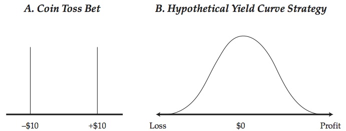
To make sense of this answer for readers who are not quantitative risk specialists, I will give a short review of options, implied volatility, and VaR. First, let’s start with VaR. Quantitative risk measurement focuses first and foremost on the P&L distribution. Consider a very simple business – flip a coin and win $10 if heads, lose $10 if tails. The P&L distribution will look like that in panel A of Figure 1 – 1/2 probability of losing $10 and 1/2 probability of winning $10. That is a complete description of the possible P&L.
P&L Distribution
But P&L for financial firms tends to look more like that in panel B – largest probability of small gain or loss, and a small probability of a large gain or large loss. (For more on this, see chapter 2 “A Practical Guide to Risk Management” or “Quantitative Risk Management”, my books on risk management) The P&L distribution is the most important item in quantitative risk measurement. If we knew the distribution we would know virtually everything there is to know about the possible P&L outcomes. But generally we don’t know or don’t care to use the whole distribution, we use summary measures – numbers that summarize the spread or dispersion of the distribution.
The two most commonly used summary measures are the volatility and the VaR (value at risk). The volatility (known to statisticians as the standard deviation) is based on the squared deviations from the mean – it measures the average deviation from the mean. The VaR (known to statisticians as a quantile) is the point on the left-hand tail of the distribution, such that there is a fixed chance of that loss or worse. (The probabilities are chosen as, say, 5% or 1% or 0.1%.) Figure 2 shows the volatility (panel A) and the 5% VaR (panel B) for the one-day P&L distribution for a hypothetical bond holding.
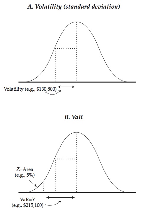
Figure 2 – Volatility and VaR for the 1-day P&L for a bond
The volatility and VaR tell us about the spread of the P&L distribution. In some cases (for example if the P&L distribution is normally-distributed) we can directly calculate the VaR from the volatility. In all cases, they both summarize the spread or dispersion and tell us about the P&L distribution, just from somewhat different perspectives.
We never know for certain what the P&L distribution will be tomorrow. We can make an informed guess or estimate what it was over some period in the past. This at least gives some basis for decision-making. (As George Santayana said, “Those who cannot remember the past are condemned to repeat it.”) The distribution in figure 2 is estimated for a holding of $20mn of the 10-year US Treasury bond as of January 2009, based on historical data from the year before.
Now we turn to the VIX and options. Consider a put option on a stock. It pays off when the stock price is below the pre-agreed strike price. Figure 3 shows the idea diagrammatically. The stock price starts at S0 today and the price may go up or down. By the expiration date it will have spread out into a distribution like shown in the diagram.
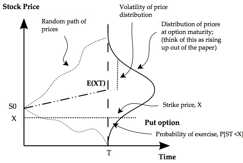
Figure 3 – Diagrammatic Representation of Option Valuation
On of the most important factors in this is the spread of the future prices, and this is measured by the volatility of the distribution. The more spread out are possible futures prices the higher the probability that the actual price will end up below the strike and the put option will be valuable.
Where does the option model volatility come from? We need to make a guess or projection of what it will be over the life of the option. If it is higher, the option price will be higher. If lower the option price will be lower.
But if we observe traded option prices in a liquid market we can back out the implied volatility – what the volatility must be to give the observed market price. In a real sense this is a market consensus volatility – what market participants think the future volatility will be, agreed by bidding and offering for options in the market. But there are two caveats. First, there may be market technical factors that push the option price higher or lower than it would otherwise be. Second, and this gets deeper into the mathematics, the distribution is the risk neutral or martingale equivalent distribution. This is subtly different from the true or objective distribution. Generally there should not be a huge difference but they will not be the same.
Now we can address more precisely whether the VIX is used in calculating the VaR. If the portfolio contained only positions in the S&P 500 index then we could use the VIX (the S&P option implied volatility) directly, subject to the two caveats above. But it will almost never be the case that a portfolio contains only the S&P index. When a portfolio contains many assets the correlations or covariance structure matters – assets will offset each other and diversify the risk.
Consider a very simple example – you hold $20mn of 10-year US Treasury and $5mn of S&P index futures. The portfolio P&L distribution (and thus the portfolio VaR) will depend on the S&P volatility, but also on the bond volatility and the correlation between the bond and the equity. The S&P volatility is one component that helps estimate the portfolio volatility and VaR, but only one.
So the short answer is, the VIX and portfolio VaR measure similar things (the spread of the price or P&L distribution) but generally for quite different portfolios (the S&P versus the assets you hold in your portfolio). While the VIX might help in estimating the portfolio VaR, it is generally only one part, and often a small part, of the overall answer.